
Two-dimensional nuclear magnetic resonance spectroscopy (2D NMR) is a set of nuclear magnetic resonance spectroscopy (NMR) methods which give data plotted in a space defined by two frequency axes rather than one. Types of 2D NMR include correlation spectroscopy (COSY), J-spectroscopy, exchange spectroscopy (EXSY), and nuclear Overhauser effect spectroscopy (NOESY). Two-dimensional NMR spectra provide more information about a molecule than one-dimensional NMR spectra and are especially useful in determining the structure of a molecule, particularly for molecules that are too complicated to work with using one-dimensional NMR.
The first two-dimensional experiment, COSY, was proposed by Jean Jeener, a professor at the Université Libre de Bruxelles, in 1971. This experiment was later implemented by Walter P. Aue, Enrico Bartholdi and Richard R. Ernst, who published their work in 1976.[1][2]

Fundamental concepts
Each experiment consists of a sequence of radio frequency (RF) pulses with delay periods in between them. It is the timing, frequencies, and intensities of these pulses that distinguish different NMR experiments from one another.[3] Almost all two-dimensional experiments have four stages: the preparation period, where a magnetization coherence is created through a set of RF pulses; the evolution period, a determined length of time during which no pulses are delivered and the nuclear spins are allowed to freely precess (rotate); the mixing period, where the coherence is manipulated by another series of pulses into a state which will give an observable signal; and the detection period, in which the free induction decay signal from the sample is observed as a function of time, in a manner identical to one-dimensional FT-NMR.[4]
The two dimensions of a two-dimensional NMR experiment are two frequency axes representing a chemical shift. Each frequency axis is associated with one of the two time variables, which are the length of the evolution period (the evolution time) and the time elapsed during the detection period (the detection time). They are each converted from a time series to a frequency series through a two-dimensional Fourier transform. A single two-dimensional experiment is generated as a series of one-dimensional experiments, with a different specific evolution time in successive experiments, with the entire duration of the detection period recorded in each experiment.[4]
The end result is a plot showing an intensity value for each pair of frequency variables. The intensities of the peaks in the spectrum can be represented using a third dimension. More commonly, intensity is indicated using contour lines or different colors.

Homonuclear through-bond correlation methods
In these methods, magnetization transfer occurs between nuclei of the same type, through J-coupling of nuclei connected by up to a few bonds.Correlation spectroscopy (COSY)

In
standard COSY, the preparation (p1) and mixing (p2) periods each
consist of a single 90° pulse separated by the evolution time t1, and
the resonance signal from the sample is read during the detection period
over a range of times t2.
The two-dimensional spectrum that results from the COSY experiment shows the frequencies for a single isotope, most commonly hydrogen (1H) along both axes. (Techniques have also been devised for generating heteronuclear correlation spectra, in which the two axes correspond to different isotopes, such as 13C and 1H.) COSY spectra show two types of peaks. Diagonal peaks have the same frequency coordinate on each axis and appear along the diagonal of the plot, while cross peaks have different values for each frequency coordinate and appear off the diagonal. Diagonal peaks correspond to the peaks in a 1D-NMR experiment, while the cross peaks indicate couplings between pairs of nuclei (much as multiplet splitting indicates couplings in 1D-NMR).[5]
Cross peaks result from a phenomenon called magnetization transfer, and their presence indicates that two nuclei are coupled which have the two different chemical shifts that make up the cross peak's coordinates. Each coupling gives two symmetrical cross peaks above and below the diagonal. That is, a cross-peak occurs when there is a correlation between the signals of the spectrum along each of the two axes at these value. One can thus determine which atoms are connected to one another (within a small number of chemical bonds) by looking for cross-peaks between various signals.[5]
An easy visual way to determine which couplings a cross peak represents is to find the diagonal peak which is directly above or below the cross peak, and the other diagonal peak which is directly to the left or right of the cross peak. The nuclei represented by those two diagonal peaks are coupled.[5]

1H COSY spectrum of progesterone
COSY-90 is the most common COSY experiment. In COSY-90, the p1 pulse tilts the nuclear spin by 90°. Another member of the COSY family is COSY-45. In COSY-45 a 45° pulse is used instead of a 90° pulse for the first pulse, p1. The advantage of a COSY-45 is that the diagonal-peaks are less pronounced, making it simpler to match cross-peaks near the diagonal in a large molecule. Additionally, the relative signs[clarification needed] of the coupling constants can be elucidated from a COSY-45 spectrum. This is not possible using COSY-90.[6] Overall, the COSY-45 offers a cleaner spectrum while the COSY-90 is more sensitive.
Another related COSY technique is double quantum filtered (DQF COSY). DQF COSY uses a coherence selection method such as phase cycling or pulsed field gradients, which cause only signals from double-quantum coherences to give an observable signal. This has the effect of decreasing the intensity of the diagonal peaks and changing their lineshape from a broad "dispersion" lineshape to a sharper "absorption" lineshape. It also eliminates diagonal peaks from uncoupled nuclei. These all have the advantage that they give a cleaner spectrum in which the diagonal peaks are prevented from obscuring the cross peaks, which are weaker in a regular COSY spectrum.[7]
Exclusive correlation spectroscopy (ECOSY)
ECOSY was developed for the accurate measurement of small J-couplings. It uses a system of three active nuclei (SXI spin system) to measure an unresolved coupling with the help of a larger coupling which is resolved in a dimension orthogonal to the small coupling.Total correlation spectroscopy (TOCSY)
The TOCSY experiment is similar to the COSY experiment, in that cross peaks of coupled protons are observed. However, cross peaks are observed not only for nuclei which are directly coupled, but also between nuclei which are connected by a chain of couplings. This makes it useful for identifying the larger interconnected networks of spin couplings. This ability is achieved by inserting a repetitive series of pulses which cause isotropic mixing during the mixing period. Longer isotropic mixing times cause the polarization to spread out through an increasing number of bonds.[8]In the case of oligosaccharides, each sugar residue is an isolated spin system, so it is possible to differentiate all the protons of a specific sugar residue. A 1D version of TOCSY is also available and by irradiating a single proton the rest of the spin system can be revealed. Recent advances in this technique include the 1D-CSSF-TOCSY (Chemical Shift Selective Filter - TOCSY) experiment, which produces higher quality spectra and allows coupling constants to be reliably extracted and used to help determine stereochemistry.
TOCSY is sometimes called "homonuclear Hartmann–Hahn spectroscopy" (HOHAHA).[9]
Incredible natural-abundance double-quantum transfer experiment (INADEQUATE)
INADEQUATE is a method often used to find 13C couplings between adjacent carbon atoms. Because the natural abundance of 13C is only about 1%, only about .01% of molecules being studied will have the two nearby 13C atoms needed for a signal in this experiment. However, correlation selection methods are used (similar to DQF COSY) to prevent signals from single 13C atoms, so that the double 13C signals can be easily resolved. Each coupled pair of nuclei gives a pair of peaks on the INADEQUATE spectrum which both have the same vertical coordinate, which is the sum of the chemical shifts of the nuclei; the horizontal coordinate of each peak is the chemical shift for each of the nuclei separately.[10]Heteronuclear through-bond correlation methods
Heteronuclear correlation spectroscopy gives signal based upon coupling between nuclei between two different types. Often the two nuclei are protons and another nucleus (called a "heteronucleus"). For historical reasons, experiments which record the proton rather than the heteronucleus spectrum during the detection period are called "inverse" experiments. This is because the low natural abundance of most heteronuclei would result in the proton spectrum being overwhelmed with signals from molecules with no active heteronuclei, making it useless for observing the desired, coupled signals. With the advent of techniques for suppressing these undesired signals, inverse correlation experiments such as HSQC, HMQC, and HMBC are actually much more common today. "Normal" heteronuclear correlation spectroscopy, in which the hetronucleus spectrum is recorded, is known as HETCOR.[11]Heteronuclear single-quantum correlation spectroscopy (HSQC)
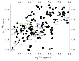
1H–15N
HSQC spectrum of a fragment of the protein NleG3-2. Each peak in the
spectrum represents a bonded N-H pair, with its two coordinates
corresponding to the chemical shifts of each of the H and N atoms. Some
of the peaks are labeled with the amino acid residue that gives that signal.[12]
Main article: Heteronuclear single-quantum correlation spectroscopy
HSQC
detects correlations between nuclei of two different types which are
separated by one bond. This method gives one peak per pair of coupled
nuclei, whose two coordinates are the chemical shifts of the two coupled
atoms.[13]HSQC works by transferring magnetization from the I nucleus (usually the proton) to the S nucleus (usually the heteroatom) using the INEPT pulse sequence; this first step is done because the proton has a greater equilibrium magnetization and thus this step creates a stronger signal. The magnetization then evolves and then is transferred back to the I nucleus for observation. An extra spin echo step can then optionally be used to decouple the signal, simplifying the spectrum by collapsing multiplets to a single peak. The undesired uncoupled signals are removed by running the experiment twice with the phase of one specific pulse reversed; this reverses the signs of the desired but not the undesired peaks, so subtracting the two spectra will give only the desired peaks.[13]
Heteronuclear multiple-quantum correlation spectroscopy (HMQC) gives an identical spectrum as HSQC, but using a different method. The two methods give similar quality results for small to medium-sized molecules, but HSQC is considered to be superior for larger molecules.[13]
Heteronuclear multiple-bond correlation spectroscopy (HMBC)
HMBC detects heteronuclear correlations over longer ranges of about 2–4 bonds. The difficulty of detecting multiple-bond correlations is that the HSQC and HMQC sequences contain a specific delay time between pulses which allows detection only of a range around a specific coupling constant. This is not a problem for the single-bond methods since the coupling constants tend to lie in a narrow range, but multiple-bond coupling constants cover a much wider range and cannot all be captured in a single HSQC or HMQC experiment.[14]In HMBC, this difficulty is overcome by omitting one of these delays from an HMQC sequence. This increases the range of coupling constants that can be detected, and also reduces signal loss from relaxation. The cost is that this eliminates the possibility of decoupling the spectrum, and introduces phase distortions into the signal. There is a modification of the HMBC method which suppresses one-bond signals, leaving only the multiple-bond signals.[14]
Through-space correlation methods
These methods establish correlations between nuclei which are physically close to each other regardless of whether there is a bond between them. They use the Nuclear Overhauser effect (NOE) by which nearby atoms (within about 5 Å) undergo cross relaxation by a mechanism related to spin–lattice relaxation.Nuclear Overhauser effect spectroscopy (NOESY)
In NOESY, the Nuclear Overhauser cross relaxation between nuclear spins during the mixing period is used to establish the correlations. The spectrum obtained is similar to COSY, with diagonal peaks and cross peaks, however the cross peaks connect resonances from nuclei that are spatially close rather than those that are through-bond coupled to each other. NOESY spectra also contain extra axial peaks which do not provide extra information and can be eliminated through a different experiment by reversing the phase of the first pulse.[15]One application of NOESY is in the study of large biomolecules such as in protein NMR, which can often be assigned using sequential walking.
The NOESY experiment can also be performed in a one-dimensional fashion by pre-selecting individual resonances. The spectra are read with the pre-selected nuclei giving a large, negative signal while neighboring nuclei are identified by weaker, positive signals. This only reveals which peaks have measurable NOEs to the resonance of interest but takes much less time than the full 2D experiment. In addition, if a pre-selected nucleus changes environment within the time scale of the experiment, multiple negative signals may be observed. This offers exchange information similar to the EXSY (exchange spectroscopy) NMR method.
NOESY experiment is important tool to identify stereochemistry of a molecule in solvent whereas single crystal XRD used to identify stereochemistry of a molecule in solid form.
Rotating frame nuclear Overhauser effect spectroscopy (ROESY)
ROESY is similar to NOESY, except that the initial state is different. Instead of observing cross relaxation from an initial state of z-magnetization, the equilibrium magnetization is rotated onto the x axis and then spin-locked by an external magnetic field so that it cannot precess. This method is useful for certain molecules whose rotational correlation time falls in a range where the Nuclear Overhauser effect is too weak to be detectable, usually molecules with a molecular weight around 1000 daltons, because ROESY has a different dependence between the correlation time and the cross-relaxation rate constant. In NOESY the cross-relaxation rate constant goes from positive to negative as the correlation time increases, giving a range where it is near zero, whereas in ROESY the cross-relaxation rate constant is always positive.[16][17]ROESY is sometimes called "cross relaxation appropriate for minimolecules emulated by locked spins" (CAMELSPIN).[17]
Resolved-spectrum methods
Unlike correlated spectra, resolved spectra spread the peaks in a 1D-NMR experiment into two dimensions without adding any extra peaks. These methods are usually called J-resolved spectroscopy, but are sometimes also known as chemical shift resolved spectroscopy or δ-resolved spectroscopy. They are useful for analysing molecules for which the 1D-NMR spectra contain overlapping multiplets as the J-resolved spectrum vertically displaces the multiplet from each nucleus by a different amount. Each peak in the 2D spectrum will have the same horizontal coordinate that it has in a non-decoupled 1D spectrum, but its vertical coordinate will be the chemical shift of the single peak that the nucleus has in a decoupled 1D spectrum.[18]For the heteronuclear version, the simplest pulse sequence used is called a Müller–Kumar–Ernst (MKE) experiment, which has a single 90° pulse for the heteronucleus for the preparation period, no mixing period, and applies a decoupling signal to the proton during the detection period. There are several variants on this pulse sequence which are more sensitive and more accurate, which fall under the categories of gated decoupler methods and spin-flip methods. Homonuclear J-resolved spectroscopy uses the spin echo pulse sequence.[18]
Higher-dimensional methods
3D and 4D experiments can also be done, sometimes by running the pulse sequences from two or three 2D experiments in series. Many of the commonly used 3D experiments, however, are triple resonance experiments; examples include the HNCA and HNCOCA experiments, which are often used in protein NMR.
Two dimensional correlation analysis is a mathematical technique that is used to study changes in measured signals. As mostly spectroscopic signals are discussed, sometime also two dimensional correlation spectroscopy is used and refers to the same technique.
In 2D correlation analysis, a sample is subjected to an external perturbation while all other parameters of the system are kept at the same value. This perturbation can be a systematic and controlled change in temperature, pressure, pH, chemical composition of the system, or even time after a catalyst was added to a chemical mixture. As a result of the controlled change (the perturbation), the system will undergo variations which are measured by a chemical or physical detection method. The measured signals or spectra will shown systematic variations that are processed with 2D correlation analysis for interpretation.
When one considers spectra that consist of few bands, it is quite obvious to determine which bands are subject to a changing intensity. Such a changing intensity can be caused for example by chemical reactions. However, the interpretation of the measured signal becomes more tricky when spectra are complex and bands are heavily overlapping. Two dimensional correlation analysis allows one to determine at which positions in such a measured signal there is a systematic change in a peak, either continuous rising or drop in intensity. 2D correlation analysis results in two complementary signals, which referred to as the 2D synchronous and 2D asynchronous spectrum. These signals allow amongst others[1][2][3]
- to determine the events that are occurring at the same time (in phase) and those events that are occurring at different times (out of phase)
- to determine the sequence of spectral changes
- to identify various inter- and intramolecular interactions
- band assignments of reacting groups
- to detect correlations between spectra of different techniques, for example near infrared spectroscopy (NIR) and Raman spectroscopy
History
2D correlation analysis originated from 2D NMR spectroscopy. Isao Noda developed perturbation based 2D spectroscopy in the 1980s.[4] This technique required sinusoidal perturbations to the chemical system under investigation. This specific type of the applied perturbation severely limited its possible applications. Following research done by several groups of scientists, perturbation based 2D spectroscopy could be developed to a more extended and generalized broader base. Since the development of generalized 2D correlation analysis in 1993 based on Fourier transformation of the data, 2D correlation analysis gained widespread use. Alternative techniques that were simpler to calculate, for example the disrelation spectrum, were also developed simultaneously. Because of its computational efficiency and simplicity, the Hilbert transform is nowadays used for the calculation of the 2D spectra. To date, 2D correlation analysis is not only used for the interpretation of many types of spectroscopic data (including XRF, UV/VIS spectroscopy, fluorescence, infrared, and Raman spectra), although its application is not limited to spectroscopy.
Properties of 2D correlation analysis

2D correlation analysis is frequently used for its main advantage: increasing the spectral resolution by spreading overlapping peaks over two dimensions and as a result simplification of the interpretation of one-dimensional spectra that are otherwise visually indistinguishable from each other.[4] Further advantages are its ease of application and the possibility to make the distinction between band shifts and band overlap.[3] Each type of spectral event, band shifting, overlapping bands of which the intensity changes in the opposite direction, band broadening, baseline change, etc. has a particular 2D pattern. See also the figure with the original dataset on the right and the corresponding 2D spectrum in the figure below.Demo dataset consisting of signals at specific intervals (1 out of 3 signals on a total of 15 signals is shown for clarity), peaks at 10 and 20 are rising in intensity whereas the peaks at 30 and 40 have a decreasing intensity
Presence of 2D spectra

2D synchronous and asynchronous spectra are basically 3D-datasets and are generally represented by contour plots. X- and y-axes are identical to the x-axis of the original dataset, whereas the different contours represent the magnitude of correlation between the spectral intensities. The 2D synchronous spectrum is symmetric relative to the main diagonal. The main diagonal thus contains positive peaks. As the peaks at (x,y) in de 2D synchronous spectrum are a measure for the correlation between the intensity changes at x and y in the original data, these main diagonal peaks are also called autopeaks and the main diagonal signal is referred to as autocorrelation signal. The off-diagonal cross-peaks can be either positive or negative. On the other hand the asynchronous spectrum is asymmetric and never has peaks on the main diagonal.Schematic presence of a 2D correlation spectrum with peak positions represented by dots. Region A is the main diagonal containing autopeaks, off-diagonal regions B contain cross-peaks.
Generally contour plots of 2D spectra are oriented with rising axes from left to right and top to down. Other orientations are possible, but interpretation has to be adapted accordingly.[5]
Calculation of 2D spectra
Suppose the original dataset D contains the n spectra in rows. The signals of the original dataset are generally preprocessed. The original spectra are compared to a reference spectrum. By subtracting a reference spectrum, often the average spectrum of the dataset, so called dynamic spectra are calculated which form the corresponding dynamic dataset E. The presence and interpretation may be dependent on the choice of reference spectrum. The equations below are valid for equally spaced measurements of the perturbation.
Calculation of the synchronous spectrum
A 2D synchronous spectrum expresses the similarity between spectral of the data in the original dataset. In generalized 2D correlation spectroscopy this is mathematically expressed as covariance (or correlation).
- Φ is the 2D synchronous spectrum
- ν1 and ν2 are two spectral channels
- yν is the vector composed of the signal intensities in E in column ν
- n the number of signals in the original dataset
Calculation of the asynchronous spectrum
Orthogonal spectra to the dynamic dataset E are obtained with the Hilbert-transform:
- Ψ is the 2D asynchronous spectrum
- ν1 en ν1 are two spectral channels
- yν is the vector composed of the signal intensities in E in column ν
- n the number of signals in the original dataset
- N the Noda-Hilbert transform matrix
- 0 if j = k
 if j ≠ k
- j the row number
- k the column number
Interpretation
Interpretation of two-dimensional correlation spectra can be considered to consist of several stages.[4]
Detection of peaks of which the intensity changes in the original dataset

As real measurement signals contain a certain level of noise, the derived 2D spectra are influenced and degraded with substantial higher amounts of noise. Hence, interpretation begins with studying the autocorrelation spectrum on the main diagonal of the 2D synchronous spectrum. In the 2D synchronous main diagonal signal on the right 4 peaks are visible at 10, 20, 30, and 40 (see also the 4 corresponding positive autopeaks in the 2D synchronous spectrum on the right). This indicates that in the original dataset 4 peaks of changing intensity are present. The intensity of peaks on the autocorrelation spectrum are directly proportional to the relative importance of the intensity change in the original spectra. Hence, if an intense band is present at position x, it is very likely that a true intensity change is occurring and the peak is not due to noise.Autocorrelation signal on the main diagonal of the synchronous 2D spectrum of the figure below (arbitrary axis units)
Additional techniques help to filter the peaks that can be seen in the 2D synchronous and asynchronous spectra.[6]
Determining the direction of intensity change

It is not always possible to unequivocally determine the direction of intensity change, such as is for example the case for highly overlapping signals next to each other and of which the intensity changes in the opposite direction. This is where the off diagonal peaks in the synchronous 2D spectrum are used for:Example of a two-dimensional correlation spectrum. Open circles in this simplified view represent positive peaks, while discs represent negative peaks
- if there is a positive cross-peak at (x, y) in the synchronous 2D spectrum, the intensity of the signals at x and y changes in the same direction
- if there is a negative cross-peak at (x, y) in the synchronous 2D spectrum, the intensity of the signals at x and y changes in the opposite direction
Determining the sequence of events
Most importantly, with the sequential order rules, also referred to as Noda's rules, the sequence of the intensity changes can be determined.[4] By carefully interpreting the signs of the 2D synchronous and asynchronous cross peaks with the following rules, the sequence of spectral events during the experiment can be determined:
- if the intensities of the bands at x and y in the dataset are changing in the same direction, the synchronous 2D cross peak at (x,y) is positive
- if the intensities of the bands at x and y in the dataset are changing in the opposite direction, the synchronous 2D cross peak at (x,y) is negative
- if the change at x mainly precedes the change in the band at y, the asynchronous 2D cross peak at (x,y) is positive
- if the change at x mainly follows the change in the band at y, the asynchronous 2D cross peak at (x,y) is negative
- if the synchronous 2D cross peak at (x,y) is negative, the interpretation of rule 3 and 4 for the asynchronous 2D peak at (x,y) has to be reversed
- where x and y are the positions on the x-xaxis of two bands in the original data that are subject to intensity changes.
It should be noted that in some cases the Noda rules cannot be so readily implied, predominately when spectral features are not caused by simple intensity variations. This may occur when band shifts occur, or when a very erratic intensity variation is present in a given frequency range.
References
- Shin-Ichi Morita; Yasuhiro F. Miura; Michio Sugi & Yukihiro Ozaki (2005). "New correlation indices invariant to band shifts in generalized two-dimensional correlation infrared spectroscopy". Chemical Physics Letters 402 (251-257): 251–257. Bibcode:2005CPL...402..251M. doi:10.1016/j.cplett.2004.12.038.
- Koichi Murayama; Boguslawa Czarnik-Matusewicz; Yuqing Wu; Roumiana Tsenkova & Yukihiro Ozaki (2000). "Comparison between conventional spectral analysis methods, chemometrics, and two-dimensional correlation spectroscopy in the analysis of near-infrared spectra of protein". Applied Spectroscopy 54 (7): 978–985. Bibcode:2000ApSpe..54..978M. doi:10.1366/0003702001950715.
- Shin-Ichi Morita & Yukihiro Ozaki (2002). "Pattern recognitions of band shifting, overlapping, and broadening using global phase description derived from generalized two-dimensional correlation spectroscopy". Applied Spectroscopy 56 (4): 502–508. Bibcode:2002ApSpe..56..502M. doi:10.1366/0003702021954953.
- Isao Noda & Yukihiro Ozaki (2004). Two-Dimensional Correlation Spectroscopy - Applications in Vibrational and Optical Spectroscopy. John Wiley & Sons Ltd. ISBN 0-471-62391-1.
- Boguslawa Czarnik-Matusewicz; Sylwia Pilorz; Lorna Ashton & Ewan W. Blanch (2006). "Potential pitfalls concerning visualization of the 2D results". Journal of molecular structure 799 (1-3): 253–258. Bibcode:2006JMoSt.799..253C. doi:10.1016/j.molstruc.2006.03.064.


References
- Aue, W. P., Bartholdi, E., and Ernst, R. R. (1976) "Two-dimensional spectroscopy. Application to nuclear magnetic resonance," Journal of Chemical Physics, 64 : 2229-46.
- Martin, G. E; Zekter, A. S. (1988). Two-Dimensional NMR Methods for Establishing Molecular Connectivity. New York: VCH Publishers, Inc. p. 59.
- Akitt, J. W.; Mann, B. E. (2000). NMR and Chemistry. Cheltenham, UK: Stanley Thornes. p. 273.
- Keeler, James (2010). Understanding NMR Spectroscopy (2nd ed.). Wiley. pp. 184–187. ISBN 978-0-470-74608-0.
- Keeler, pp. 190–191.
- Akitt & Mann, p. 287.
- Keeler, pp. 199–203.
- Keeler, pp. 223–226.
- "2D: Homonuclear correlation: TOCSY". Queen's University. Retrieved 26 June 2011.
- Keeler, pp. 206–208.
- Keeler, pp. 208–209, 220.
- Wu, Bin; Skarina, Tatiana; Yee, Adelinda; Jobin, Marie-Claude; DiLeo, Rosa; Semesi, Anthony et al. (June 2010). "NleG Type 3 Effectors from Enterohaemorrhagic Escherichia coli Are U-Box E3 Ubiquitin Ligases". PLoS Pathogens 6 (6): e1000960. doi:10.1371/journal.ppat.1000960.
- Keeler, pp. 209–215.
- Keeler, pp. 215–219.
- Keeler, pp. 274, 281–284.
- Keeler, pp. 273, 297–299.
Boracay islands, Philippines
Boracay islands, Philippines

Boracay - Wikipedia, the free encyclopedia
en.wikipedia.org/wiki/Boracay


///////
No comments:
Post a Comment